A special thanks to Jack Cheng for his contributions to this blog post.

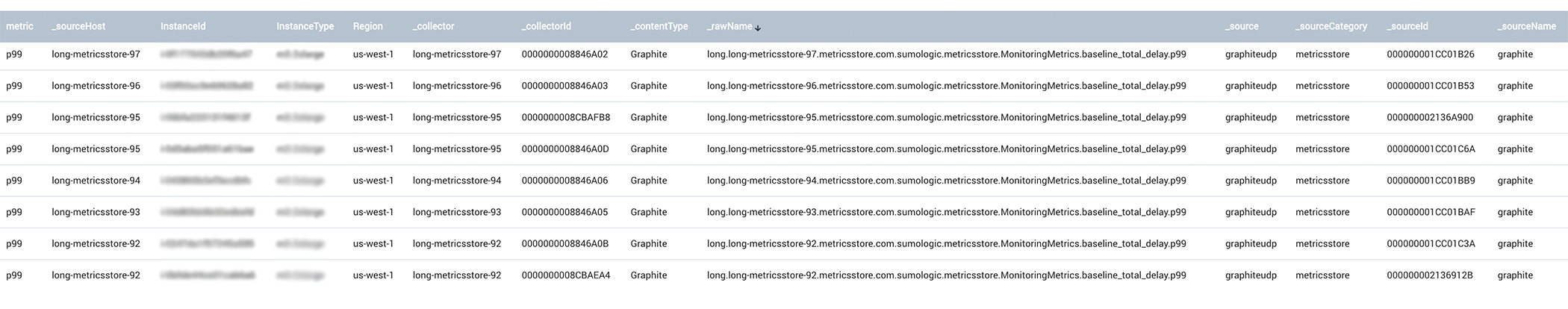
Imagine waking up at 3 a.m. to a pager alert, and looking at the below graph. You are trying to determine which host that spike came from. Unfortunately, the legend on the right margin is severely truncated and stubbornly refuses to offer any help. So you turn to the tooltip, only to be greeted with the clutter of 20 odd pieces of metadata that collectively identify your target. You squint hard and are finally able to locate the _sourceHost in the tooltip, but you start to feel that this is going to be a long night.

Figure 1

Phew!

This situation isn’t uncommon when you are charting large volumes of multi-dimensional data. In fact, this is how legends used to look in some of the earliest prototypes of our Sumo Logic Metrics solution. We have come a long way since then; Sumo Logic Metrics now automatically creates legends and tooltips that are more concise and informative, making it easier to quickly make sense of your data. However, along the way, we discovered that the general problem of selecting the “best” (as per one intuitively plausible criterion) legend is computationally hard.

In this blog post, we would like to share these findings with you. We will describe our formulation of the problem, share our insights into its computational complexity and talk about our experiences in practice.

Concision and Precision

Let’s revisit the example from above, and see why legends there are hard to understand.

The graph contains close to a 100 time-series, and each series is described by about 20 different key-value pairs of metadata.

Figure 2

That’s a lot of data to take in if we are trying to quickly understand what each time-series represents. But volume comes in the way of comprehension in more respects than one. It also distracts from and clouds out the relevant bits. In the example, the tags _sourceHost, InstanceId, and collectorId seem to carry most of the information a user would typically want to see for this graph. But these tags get drowned out in the sea of other, less informative, tags such as _sourceCategory, InstanceType, and _collectorId.

We present two qualitative criteria to help define what makes a legend informative and useful: conciseness and precision.

A legend is concise when it includes enough information to describe the items being labelled, and nothing more.

Another, and even more important, property we want from legends is their precision — the ability to unambiguously identify an item from its label. Little can be made of a pair of labels in a graph that are identical to each other.

Concision and precision can compete with each other. The legend in Figure 2 includes every key present, and is therefore very precise. In contrast, consider another legend that shows only, say, _sourceCategory tags. Such a legend would be very concise. But it would also reduce every time-series to the same label, and therefore wouldn’t be at all precise.

How does one find the most concise legend that is precise?

There are far too many combinations of keys—$$2^\text{\# of keys}$$, to be exact — to individually check for precision. Can we do better? Something in steps polynomial in the number of keys? The answer is, most likely, no. As we show next, the problem of finding the most concise discriminating legend is NP-hard.

Minimal Legend Selection

In the remainder of this post, we will concern ourselves with only the metadata of time-series, ignoring such aspects as data points and timestamps. We will consider each time-series as being a metadata item $$t$$, given in the form of a map of key-value pairs:

$$t ~:=~ \{k_1 \mapsto v_1, \dotsc, k_n \mapsto v_n\}$$

We will use the notation $$t.k$$ to refer to the value $$v$$ for which $$k \mapsto v$$ appears in the map, or $$\textsf{null}$$, if there is no such value.

Interchangeably, we will occasionally think of these items as being functions $${\cal K} \rightarrow {\cal V}$$, with $${\cal K}$$ and $${\cal V}$$ representing the universe of keys and values, respectively. (Note: Items may not map each key to a value. To accommodate such cases, we assume our universe of values contains a special ‘null’ value, that each of the missing keys in an item map to.)

Given a set of keys $$K \subseteq {\cal K}$$, the label wrt. $$K$$ of an item $$t$$ is the projection denoted by

$$t|_K ~:=~ \{k \mapsto t.k ~|~ k \in K\}$$

Given a set of items $$T = \{t_1, \dotsc, t_n\}$$, and a set of keys $$K$$, we refer to the number of unique labels that $$K$$ produces as its precision for $$T$$. And we say $$K$$ is discriminating for $$T$$ if it has the maximum precision for $$T$$, i.e., if the 2 sets have the same cardinality:

$$|\{t_1, \dotsc, t_n\}| = |\{t_1|_K, \dotsc, t_n|_K\}|$$

A set of keys that is discriminating for a set of items produces unique labels for each item.

Finally, given the tuple $$\big({\cal K}\colon \text{Set}, {\cal V}\colon \text{Set}, T\colon \text{Set}[{\cal K} \rightarrow {\cal V}]\big)$$, the Minimal Legend Selection (MLS) problem is to find a subset of keys $$K \subseteq \cal{K}$$ such that the following hold:

1. $$K$$ is discriminating for $$T$$, and
2. There is no smaller subset of keys discriminating for $$T$$. (Note: There may be more than 1 subset of discriminating keys that are both minimal. Consider, for example, a set of time-series where each _sourceHost corresponds to a unique InstanceId, and vice-versa. In such a case, we can swap one key for another in a legend without loss of its discriminatory power. Choosing between different minimal legends is an interesting topic, but is out of scope of this article.) That is, for any $$K‘$$ that is discriminating for $$T$$, it is the case that $$|K‘| \geq |K|$$.

Thus, the Minimal Legend Selection seeks to find the smallest set of keys we can show in the legend that provide enough information to tell the series apart.

Minimal Legend Selection is NP-hard

Minimal Legend Selection is NP-hard. To demonstrate, we present a polynomial-time reduction of the Set Cover problem to Minimal Legend Selection.

First, let’s recall that in the set cover problem $$\big(U, {\cal S}\big)$$, we are given

• A universe of elements $$U = \{e_1, \dotsc, e_n\}$$, and
• A collection of subsets $${\cal S} = \{S_1, \dotsc, S_m \}$$, $$S_i \subseteq U$$, that covers $$U$$

and we wish to find a sub-collection $${\cal C} \subseteq {\cal S}$$ containing the fewest subsets that covers $$U$$:

$$\displaystyle\bigcup_{S_i \in {\cal C}} S_i ~=~ U$$

Reduction from Set Cover

In order to phrase a Set Cover problem $$\big(U, {\cal S}\big)$$ as a Minimal Legend Selection problem, we shall consider:

1. Each element $$e \in U$$ as being a time-series, and
2. Each subset $$S \in {\cal S}$$ as corresponding to a key and describing the discriminated pairs of time-series for the key. We set up values for the key $$S$$ such that
3. Each time-series in $$S$$ is given a unique value, and
4. Time-series that are not in $$S$$ are all assigned the same value. We will refer to this value as $$\star$$.

Finally, we add a time-series $$\bigstar$$ that takes the value $$\star$$ along each key $$S \in {\cal S}$$. Note that due to the fact that $${\cal S}$$ covers $$U$$, $$\bigstar$$ is guaranteed to be different from every $$e \in U$$.

We now present the reduction mechanics formally. Given a Set Cover problem $$\big(U = \{e_1, \dotsc, e_n\}, {\cal S} = \{S_1, \dotsc, S_m\}\big)$$, we construct an instance of Minimal Legend Selection $$({\cal K}, {\cal V}, T)$$ where:

• The set of keys $${\cal K} = \{1, \dotsc, m \}$$, i.e., one key for each $$S$$.
• The set of values $${\cal V} = \{1, \dotsc, n, \star\}$$, i.e., one value for each item.
• The set of items $$T = \{1, \dotsc, n, \bigstar\}$$, i.e., one for each element and a special item
• With the key-value mapping being:

It is straightforward to verify that a minimal legend in this setup corresponds to a minimal set cover in the original Set Cover problem.

Claim 1

A discriminating legend for $$\big({\cal K}, {\cal V}, T\big)$$ is a set cover for $$\big(U, {\cal S}\big)$$.

Proof: Let $$K$$ be a discriminating legend. For any given $$e_i \in U$$, there exists a key $$j \in {\cal K}$$ that distinguishes $$i$$ from $$\bigstar$$, i.e., $$i.j \not= \star$$. It must be the case that $$e_i \in S_j$$.

Claim 2

A set cover for $$\big(U, {\cal S}\big)$$ is a discriminating legend for $$\big({\cal K}, {\cal V}, T\big)$$.

Proof: Let $$i$$ and $$j$$ be distinct arbitrary items in $$T$$. W.l.o.g., let $$i$$ be the item that is not $$\bigstar$$, and let $$S_k$$ be a subset in the given set cover that contains $$e_i$$. By construction, the key $$k$$ distinguishes $$i$$ from $$j$$.

Corollary

A minimal legend selection for $$\big({\cal K}, {\cal V}, T\big)$$ is a minimal set cover for $$\big(U, {\cal S}\big)$$.

Proof: Claim 1 shows that a minimal discriminating legend is a set cover. Minimality of this cover follows from Claim 2—a smaller set cover yields a smaller discriminating set in MLS thus contradicting our hypothesis.

Minimal Legend Selection as an Optimization Problem

We showed above that Minimal Legend Selection is NP-hard. Unless it turns out that P = NP, exact solutions to MLS are going to be prohibitively expensive to compute. We now look at an Integer Linear Program (ILP) for a Minimal Legend Selection that can be relaxed in practice to arrive at an approximate solution to the problem.

Let $$T = \{t_1, \dotsc, t_n\}$$ be the set of given time-series, and $${\cal K} = \{k_1, \dotsc, k_m\}$$ be the set of keys appearing in $$T$$.

For each key $$k_i \in \cal{K}$$, and each pair $$t_p, t_q$$ of time-series in $$T$$, let $$\Delta_{p,q}^{i}$$ denote whether the key $$k_i$$ differentiates $$t_p$$ from $$t_q$$:

The Minimal Legend Selection problem can now be formulated as the 0-1 ILP:

Concluding Remarks

Despite the intractability of the general problem of finding minimal legends for a given set of time-series, the situation isn’t so grim in practice. In addition to query results, we use heuristics to bring additional pieces of information to bear on the problem of legend selection. For example, by analyzing search terms for wildcard-like patterns, we are able to directly infer some or all of the discriminating keys in a large number of selector-only queries. Search term analysis benefits aggregate-style queries too, where the discriminating legend can be created from the grouping keys used in the final aggregate operator.

In practice, minimality isn’t our only concern when selecting a legend; we also try to improve legend relevance by bringing in contextual information about the various keys. This allows us to, for instance, treat a human-readable dimension such as _sourceHost preferentially in comparison to a hexadecimal-valued _sourceId, whenever there is a choice. A full discussion of this is outside the scope of this blog post.

Lastly, for the times when the user might want a certain key to show up in the legends, regardless of minimality, or when they want to craft the legend in a particular way, we provide Custom Labels. This allows the user to hand-craft a labelling scheme using string-concatenation of keys and values.

Additional Resources

• Learn how to evaluate React Table alternatives.
• Want to better understand Sumo Query Language design patterns?
• Postmortems and outages getting you down? Read why software engineers should learn to embrace these instead of dread them!

Guest Author Bio

Jack Cheng is a senior software engineer at LogicHub, working on the decision engine that helps customers derive insights from their data and automate actions from those insights. In his free time, he solves algorithm and math puzzles. Prior to LogicHub, Jack was a software engineer at Sumo Logic.